Turbulence: Harmony of Primes Under the Mask of Chaos
Unlocking the Secret Box:
Why Turbulence is Not Chaos, but a Symphony of Primes
“God does not play dice with the universe.”
“When I meet God, I am going to ask him two questions: Why relativity? And why turbulence? I really believe he will have an answer for the first.”
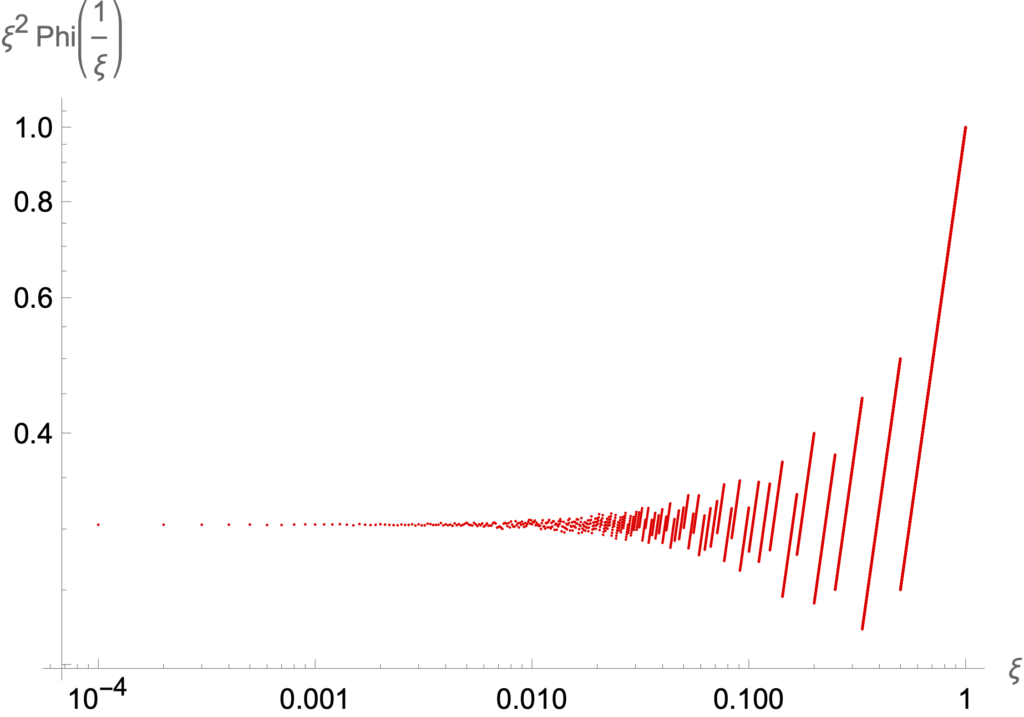
“The turbulence of number theory is the statistics of the values of the Euler function \(\varphi(n)\)… This is a very intermittent sequence.”
For centuries, humanity has stared at the rushing white water of a river, the swirling exhaust of a jet engine, or the violent storms of Jupiter, and accepted a fundamental assumption: This is absolute chaos.
To explain this chaotic mess, the phenomenological theory of turbulence assumed “spontaneous stochasticity.” For the last fifty years, the global physics and engineering communities believed that as you zoom in on a turbulent fluid, it becomes a continuous, random “multifractal” cascade. To simulate fluid flow, scientists inject random noise into their supercomputers, hoping that if they roll the dice enough times, the math will smooth out into a continuous probability distribution.
They thought Mother Nature was a gambler.
But exactly one hundred years ago, in 1926, Albert Einstein famously warned us: “God does not play dice.” For a century, the fluid dynamics community believed that in the macroscopic world of turbulence, He did.
Using a mathematical skeleton key I developed called Loop Calculus, I have finally picked the lock on the exact 3D Navier-Stokes equations to see exactly what is inside the secret box of turbulence.
When we open the box, we discover something breathtaking: Einstein was right. There are no dice.
Chaos vs. The Farey Sequence
The “chaos” we see with our naked eyes is a magnificent optical illusion. Turbulence is not a random, statistical phenomenon. There are no continuous multifractal scaling laws. Instead of rolling dice, the fluid is computing exact, discrete arithmetic.
The spatial structure of turbulence is mapped exactly onto a deterministic number-theoretic object known as the Farey sequence. What is the difference? Imagine you are trying to intercept an encrypted computer file. To the naked eye, the data looks like pure, erratic gibberish. That is chaos.
A Farey sequence of order \(n\), denoted as \(F_n\), is the strictly ordered sequence of completely reduced rational fractions between \(0\) and \(1\) whose denominators do not exceed \(n\). For example, the Farey sequence of order 5 is the ordered set:
\[ F_5 = \left\{ \frac{0}{1}, \frac{1}{5}, \frac{1}{4}, \frac{1}{3}, \frac{2}{5}, \frac{1}{2}, \frac{3}{5}, \frac{2}{3}, \frac{3}{4}, \frac{4}{5}, \frac{1}{1} \right\} \]
Because these fractions are built entirely out of coprime integers, the sequence jumps and stutters in highly specific ways. The sudden, violent bursts and quiet lulls in a turbulent fluid—what physicists call “intermittency”—are not random statistical outliers. They are the physical manifestation of the exact mathematical gaps between these ordered rational numbers.
In pure mathematics, the intermittency of the Farey sequence is so profound that its fluctuations were proven to be directly related to the Riemann Hypothesis. By forcing continuous fractal power-laws onto turbulence, the establishment has been actively trying to smooth over an encrypted discrete code. The fluid isn’t calculating continuous, floating-point random variables; it is calculating exact rational fractions.
A String Theory in Dual Fourier Space
How does a physical fluid compute these fractions? Turbulence is driven by violently swirling 3D vortices forming closed liquid loops. In my exact solution, I utilize Loop Calculus to represent the fluid dynamics as a string theory of these interacting vortex loops.
However, unlike the continuous spacetime assumed in fundamental physics, this formulation possesses a strictly discrete target space. To be mathematically precise: you will not find rigid geometric polygons splashing around in the physical water. This discrete target space exists entirely in the dual Fourier description (the Fourier loop space) that mathematically describes the moving liquid loops.
In this dual Fourier space, the target space consists of regular star polygons—geometric figures (like an equilateral triangle, a square, or a five-pointed star) whose vertex angles are exact rational fractions of \(2\pi\).
While the physical water flows continuously, its underlying harmonic architecture in momentum space is locked into a discrete geometric lattice of polygonal vortex strings. Their interactions are perfectly governed by the rational fractions of the Farey sequence, generating the extreme intermittent bursts we observe in the physical fluid.
Euler’s \(\varphi(n)\) and the Code of Nature
To understand how simple fractions create the illusion of physical chaos, we must look at a mathematical object called Euler’s totient function, denoted as \(\varphi(n)\). As V.I. Arnol’d brilliantly observed in 1993, this function is the true source of “turbulence” in number theory.
In simple terms, \(\varphi(n)\) counts the number of completely reduced fractions that have a specific denominator \(n\) (this is exactly the number of new fractions added to the Farey sequence for that denominator). Euler discovered a beautiful, exact formula for this function:
\[ \varphi(n) = n \prod_{p_k | n} \left(1 – \frac{1}{p_k}\right) \]
where the product is taken over all unique prime factors \(p_k\) that divide \(n\).
Look closely at this formula. There is no randomness here. The “chaos” arises entirely from the prime factorization of \(n\)—the exact same mathematical mechanism that secures modern computer cryptography. Because the distribution of prime divisors jumps wildly from one number to the next, plotting \(\varphi(n)\) creates a scatter of points that looks like a chaotic spray, yet is perfectly deterministic.

The Hidden Harmony of Primes and Zeta Zeros
Because turbulence is governed by these exact fractions, the overall physics of fluid flow is intimately tied to the Riemann zeta function, \(\zeta(s)\)—the master analytic function that governs the distribution of prime numbers.
In my exact analytic solution, the energy spectrum of decaying turbulence doesn’t follow an arbitrary, phenomenologically fitted curve. It decays according to an exact, beautiful law derived directly from number theory:
\[ E \propto t^{-5/4} \]
For exactly sixty years, since the historical experiments of Comte-Bellot and Corrsin in a water pipe with an oscillating grid in 1966, this “\(5/4\)” scaling law was observed in empirical physics and recently confirmed in large scale supercomputer simulations. Its theoretical origin was a total mystery. Now, we know it is an exact theorem. This fractional exponent is explicitly derived from the Riemann zeta function evaluated at zero:
\[ \frac{5}{4} = 1 – \frac{\zeta(0)}{2} \]
(Since the zeta function evaluates to \(\zeta(0) = -1/2\), the pure arithmetic yields exactly the physical \(5/4\) decay rate observed in nature).
But the connection goes even deeper. My exact geometric theory predicts that the effective index (the logarithmic derivative) of the velocity correlation as a function of separation distance does not decay monotonically. Instead, it exhibits distinct oscillations.
My solution relates these exact spatial oscillations directly to the complex zeros of the Riemann zeta function. Stunningly, such spatial oscillations in the velocity correlation were indeed observed in physical wind tunnel experiments at the Max Planck Institute Turbulence Center. Mother Nature was physically computing the complex zeros of the zeta function inside their wind tunnel!
We can actually see this hidden harmony of primes. In my recent paper on the exact solution of turbulent mixing (such as a drop of dye in a turbulent fluid, known as a passive scalar), the analytical formulas produce a stunning visual signature: an Arithmetic Matrioshka doll made of an infinite number of concentric spherical shells, condensing to the center.
The physical fluid exactly mirrors the arithmetic of its dual space. The “chaos” of the dye shredding in the water is just the physical manifestation of the exact discrete lattice operating in Fourier loop space, perfectly fulfilling V.I. Arnol’d’s prophetic intuition from 1993. These discrete shells and extreme intermittent spikes do not have a continuum limit. They do not converge into a smooth curve. They are the strict, deterministic footprints of prime numbers.
We thought turbulence was the ultimate physical mess—a triumph of randomness over order. It turns out, it is the ultimate mathematical symphony. The centuries-old Enigma of turbulence has not been solved by adding more random noise to a bigger supercomputer. It has been solved by realizing that Mother Nature is a Number Theorist.
The Mathematical Proofs & Historical Context
The mathematical details of these discoveries, along with their empirical supercomputer confirmations, will be published this spring as a series of invited papers in the Philosophical Transactions of the Royal Society A. It is a historical symmetry that this is the exact same scientific journal that published Isaac Newton’s foundational works on Calculus and classical mechanics in the 17th century.
For physicists, mathematicians, and fluid dynamicists who wish to examine the exact Loop Calculus, the continuous-to-discrete mappings, and the empirical data, the comprehensive preprints and historical context are currently available below:
- Migdal, A. “Geometric Solution of Turbulence as Diffusion in Loop Space.”
(Derivation of the exact solution of decaying turbulence in the 3D Navier-Stokes equation, introducing the Farey sequence, the string theory of star polygons in Fourier loop space, and arithmetic intermittency).
Invited paper to Phil. Trans. R. Soc. A. Preprint: arXiv:2511.02165 - Migdal, A. “Geometric Solution of Turbulent Mixing.”
(The exact solution of the passive scalar, deriving the spherical shell structures and spatial density distributions).
Invited paper to Phil. Trans. R. Soc. A. Preprint: arXiv:2504.10205 - Rodhiya, A., Sreenivasan, K. R. “The Asymptotic State of Decaying Turbulence.”
(A comprehensive Direct Numerical Simulation independently confirming the exact \(5/4\) asymptotic decay state predicted by the geometric theory).
Invited paper to Phil. Trans. R. Soc. A. Preprint: arXiv:2602.12501 - K.R. Sreenivasan. “Decaying Turbulence”, Joint SOM/SNS HEP seminar in the Institute for Advanced Study, April 6, 2026. https://youtu.be/-wDtx8CEK2A?si=5bNx36clLO1Xdn0C
- Comte-Bellot, G., Corrsin, S. “The use of a contraction to improve the isotropy of grid-generated turbulence.”
Journal of Fluid Mechanics. 1966; 25(4):657-682. © 1966 Cambridge University Press.
(The historic 1966 experiment measuring decaying turbulence created by an oscillating grid in a water pipe, which first definitively captured the mysterious \(5/4\) decay exponent in physical space, exactly 60 years before it was mathematically proven to originate from the Riemann zeta function).