Quantum Pendulum of Classical Turbulence
“Turbulence is an essentially statistical problem of the same type as one meets in statistical mechanics, since it is the problem of distribution of energy among a very large number of degrees of freedom.”
— Werner Heisenberg (1948)
For more than a century, turbulence has guarded its deepest secret behind a veil of apparent chaos. We see it in the curl of rising smoke, the wake of a ship, and the churning atmosphere of a planet—a deterministic classical fluid governed by the Navier–Stokes equations, yet dissolving at high Reynolds numbers into an endlessly intricate cascade of eddies. Phenomenology offered scaling laws, which turned out to be only approximate; no quantitative theory of turbulence was ever found. What remained was the central question a theoretical physicist asks first: what is the probability distribution of a turbulent flow, the true counterpart of the Gibbs distribution in statistical mechanics?
Here lies a remarkable historical irony. In 1948, having helped create quantum mechanics, Werner Heisenberg turned his gaze to classical fluid dynamics and envisioned a simple Boltzmann–Gibbs distribution of energy among classical vortex structures and fluid degrees of freedom. He set quantum theory aside in search of a classical statistical ensemble in physical space—never suspecting that the exact solution of classical turbulence would lead straight back to a quantum-mechanical Gibbs distribution. What would Heisenberg say if he were told that the secret energy distribution of decaying turbulence is governed by the quantum mechanics of a pendulum?
In The quantum pendulum of turbulent flow: Decaying turbulence as a thermal state of an integrable system, I show that the turbulent attractor lives in a Hilbert space and is mathematically equivalent to a pair of quantum pendulums. In short, the statistics of vorticity in decaying turbulence reduce explicitly to the quantum Gibbs state \(\exp(-\beta_{\text{eff}} H)\) of a pendulum system with the Mathieu Hamiltonian \(H = -\frac{1}{2}\partial_\theta^2 + \frac{b^2}{8}\sin^2\theta\). The effective inverse temperature \(\beta_{\text{eff}}\) is distributed with an explicit weight, and the vorticity correlations are an integral transform of this statistical average. Once this quantum-mechanical correspondence is recognized, the problem reduces to the Mathieu equation—the simplest known solvable nonlinear quantum system. Even more remarkably, this hidden equivalence is now a proven theorem, formally verified in Lean 4 in a forthcoming joint paper with the Google Research team.
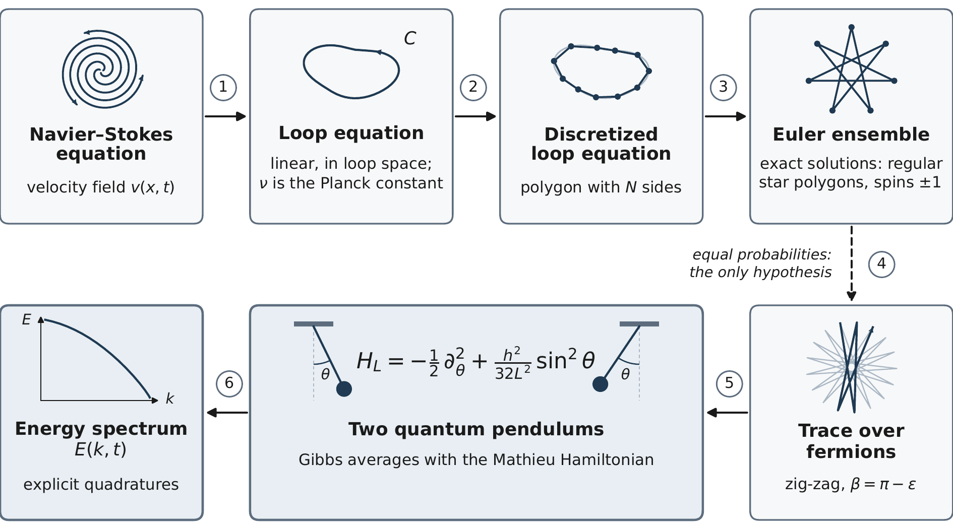
The path of the solution, from the Navier–Stokes equations to the energy spectrum. Solid arrows indicate exact mathematical transformations, definitions, or theorems; the dashed arrow marks the single physical hypothesis—the equal probability of all states in the Euler ensemble.
From Interacting Eddies to Quantum Operators
While this perspective may be difficult to digest for traditional turbulence modelers focused on interacting eddies in physical flow, those interacting eddies are mathematically represented by quantum-mechanical operators in dual momentum loop space. This conceptual shift is directly analogous to Lars Onsager’s celebrated solution of the two-dimensional Ising model, where strongly coupled \(\pm 1\) classical spins are represented as free Majorana fermions in a dual quantum description.
The foundation of this duality goes back to the loop equation I established in 1993. Instead of following the velocity at isolated points in space, we track the circulation \(\Gamma_C\) around a closed contour \(C\) and its average exponential, the loop functional \(\Psi[C] = \langle \exp(i\Gamma_C/\nu) \rangle\). Incompressibility and pressure elimination are built directly into this observable, and the nonlinear Navier–Stokes dynamics becomes a linear evolution equation in loop space. Along the contour, the loop parameter acts as time, the kinematic viscosity \(\nu\) plays the role of Planck’s constant, vorticity arises as the commutator of covariant derivatives, and the loop functional itself is a quantum amplitude. Regularizing the contour as a closed polygon of \(N\) sides—an ultraviolet lattice cutoff—and taking the continuum limit \(N \to \infty\) at fixed turbulent viscosity \(\tilde{\nu}\) defines the turbulent attractor.
The Euler Ensemble and Noise-Triggered Ergodicity
Mapping the discretized loop equation into momentum loop space turns it into an algebraic system with an exact manifold of decaying solutions: the Euler ensemble. Its states are regular star polygons in a complex three-dimensional space, labeled by a rational turning angle and a periodic chain of \(N\) Ising spins \(\pm 1\) with zero net winding. On every polygon in this manifold, the viscous and advective terms vanish separately.
Yet individual Euler polygons are linearly unstable under the deterministic loop flow: on the zero-winding manifold, the time-derivative matrix becomes singular, so an arbitrarily faint perturbation—the background thermal agitation present in every real fluid—triggers a random walk across the Euler states. Modeling this noise-triggered motion through minimal-impulse swaps of neighboring spins and reflected shifts of the turning angle yields a symmetric Markov process governed by a proven H-theorem: entropy grows monotonically until all Euler states carry equal weight. This microcanonical equidistribution, the loop-space counterpart of Boltzmann’s ergodic hypothesis, is the single physical postulate of the theory.
From Fast Spins to the Quantum Pendulum
To measure the correlation of vorticity at two points in space, we deform the loop into a narrow hairpin passing through both points. Rewriting the equal-weight sum over spin chains as a quantum trace over lattice fermions reveals a striking separation of scales near the critical zig-zag turning angle \(\beta = \pi\): pairs of opposite spins act as a fast thermal bath for the slowly wandering orientation of the polygon. In the continuum limit \(N \to \infty\), the closed loop becomes a thermal circle in Euclidean imaginary time, and the two arcs of the hairpin crystallize into two quantum pendulums. Their quantum Gibbs distribution is not postulated—it is born dynamically from the uniform weight of the Euler states, much as the Hawking temperature emerges from the horizon geometry of a black hole without an external heat bath.
This reduction supersedes my earlier finite-\(N\) saddle-point picture. When \(N \to \infty\), the intricate number-theoretic structure of rational turning angles—Euler’s totient function, Farey fractions, and the earlier conjecture involving Riemann zeta zeros—washes out into a smooth continuum density. What endures is pure geometry and integrable quantum mechanics, predicting a universal short-distance enstrophy ratio of \(1/8\).
A Surprising Singularity in the Energy Spectrum
Perhaps the most unexpected physical prediction of the quantum pendulum solution is a sharp singularity hidden inside the decaying energy spectrum \(E(k, t)\). Because time and wavenumber enter the pendulum Hamiltonian solely through the dimensionless combination \(kL(t)\), where \(L(t) = \sqrt{\tilde{\nu}(t + t_0)}\) is the growing viscous length scale, hairpins divided into two equal arcs create a critical threshold at \(kL(t) = \sqrt{2}\).
Across this threshold, the energy spectrum stays continuous, but its slope diverges as a double logarithm. Viewed at any fixed wavenumber \(k\) as the turbulence decays and \(L(t)\) expands, the flow passes through a genuine finite-time singularity at the critical instant \(t_*(k) = \frac{2}{\tilde{\nu}k^2} – t_0\), where the time derivative \(\partial_t E(k, t)\) diverges as the viscous scale sweeps across \(\sqrt{2}/k\). Transformed back into physical space, this spectral threshold materializes as a coherent spatial wave: the two-point vorticity correlation oscillates with a universal period \(\sqrt{2}\,\pi L(t) \simeq 4.44\,L(t)\)—a macroscopic echo of integrable quantum dynamics ringing inside decaying classical chaos.
A Theorem Verified by AI in Lean 4
In collaboration with the Google Research team—Yanchen Jiang, Michael P. Brenner, Yang Cai, Vineet Gupta, Kaylie Hausknecht, Christopher Liaw, Aranyak Mehta, Grigoris Velegkas, and Di Wang—we used Google Research’s multi-agent proof harness Cogentic together with the Lean 4 interactive theorem prover to turn the entire derivation into a machine-verified mathematical theorem. The formal proof spans roughly 760,000 lines of Lean 4 code and verifies 95 target theorems across six packages.
This human–AI collaboration went far beyond checking steps already on paper: automated proof search and kernel verification uncovered and resolved the subtle non-commutativity between the infinite-polygon limit \(N \to \infty\) and the short-distance limit \(h \to 0^+\), supplying the Toeplitz-commutator estimate needed to prove the \(1/8\) enstrophy law unconditionally, alongside explicit convergence rates and closed-form pendulum constants.
Heisenberg foresaw that the riddle of turbulence belonged to statistical mechanics, expecting a classical Gibbs distribution over classical vortex structures. Nature’s answer turned out to be far more subtle: in momentum loop space, the dissipative chaos of a classical fluid is governed by the quantum-mechanical Gibbs distribution of an integrable pendulum—a bridge between classical and quantum physics now standing as a machine-verified theorem.
References
- Alexander Migdal, “The quantum pendulum of turbulent flow: Decaying turbulence as a thermal state of an integrable system,” arXiv:2607.05745v6 (2026).
- Yanchen Jiang, Alexander Migdal, Michael P. Brenner, Yang Cai, Vineet Gupta, Kaylie Hausknecht, Christopher Liaw, Aranyak Mehta, Grigoris Velegkas, and Di Wang, “Proof of Migdal’s Quantum Pendulum Solution of Decaying Turbulence,” Google Research & Institute for Advanced Study (forthcoming, 2026).